Top 3 Excel Formatting Tips and Tricks for Better Data Presentation
Spreadsheets shouldn’t be dull and dry — if you want people to read them, that is. Learn a few tricks to make formatting your data easy and create Excel workbooks that get engagement from your colleagues.
Formatting Tricks in Excel 1: Using the Fill Handle
Step 1: Open an existing Excel workbook. Here we have an unfinished table showing profits for a small business.
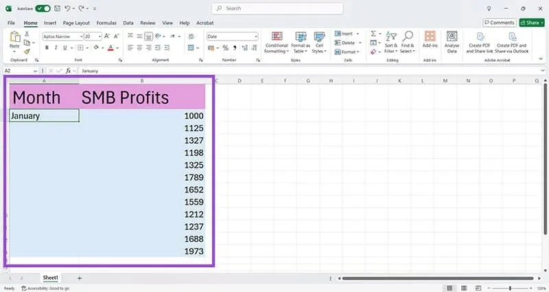
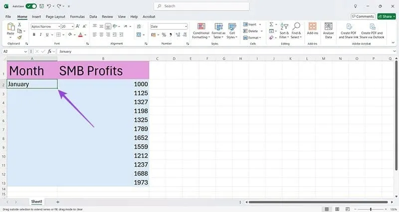
Step 2: To complete the Month column without typing manually, click cell A2 (January) and hover the cursor over the bottom right corner to reveal the fill handle, a small black plus sign.
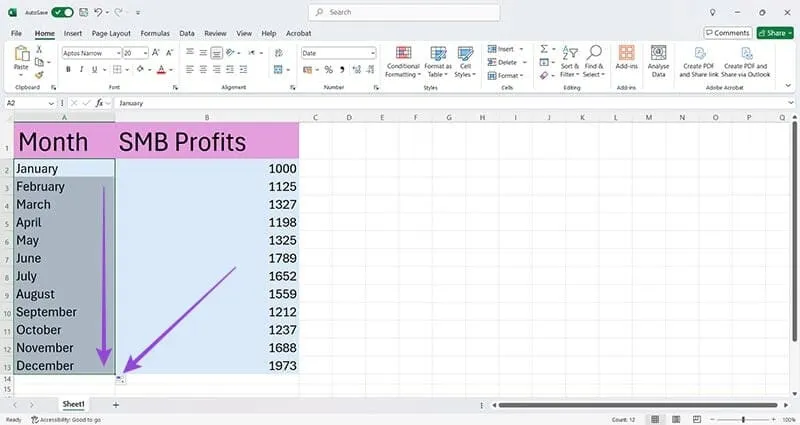
Step 3: Drag the fill handle down to cell A13 to fill the months in order. For extensive lists, double-click the fill handle to complete entries automatically.
Formatting Tricks in Excel 2: Number Formatting
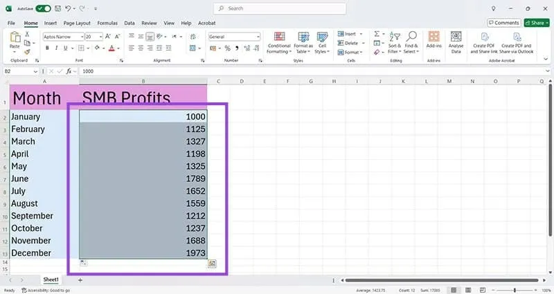
Step 1: Select the Profits column, which currently lacks currency formatting.
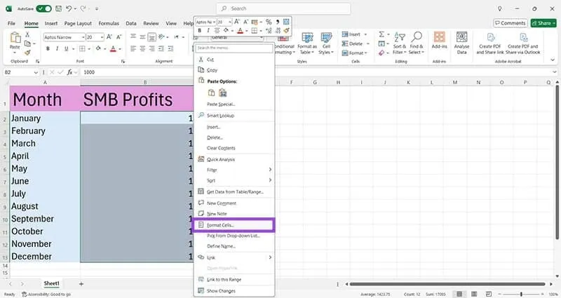
Step 2: Right-click the selected cells and choose Format Cells.
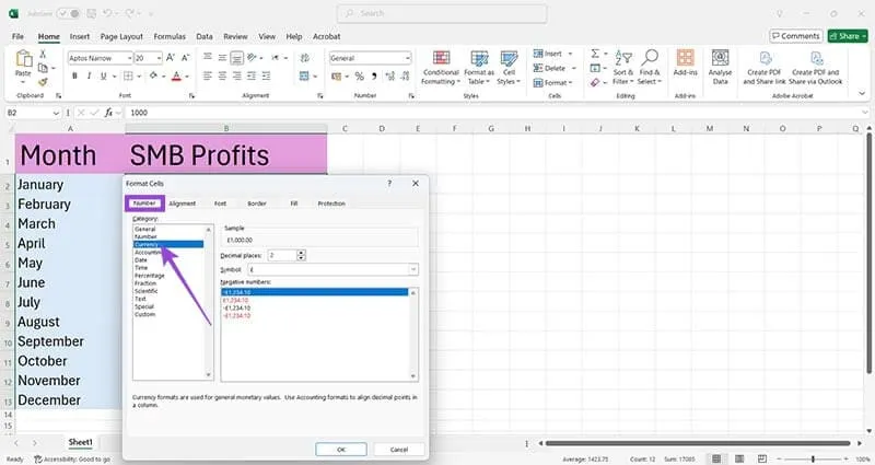
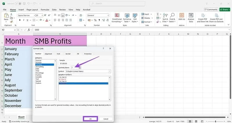
Step 3: In the Format Cells window, select Currency under the Number tab.
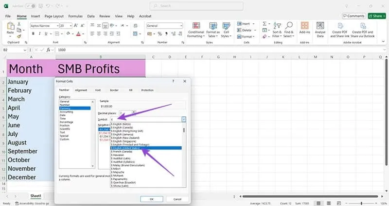
Step 4: Choose your desired currency symbol (e.g., US dollars), adjust decimal places to 2, and select how negative amounts should appear.
Step 5: Click OK to transform the numbers into formatted currency automatically.
Formatting Tricks in Excel 3: Adding Graphics to Data
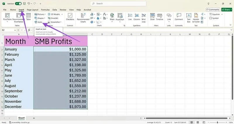
Step 1: Click on the Insert tab and then select Icons to open a graphics library.
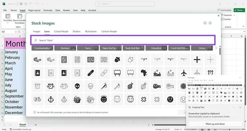
Step 2: Browse the available icons or use the search bar to find suitable graphics.
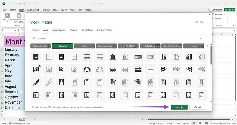
Step 3: Click on icons you want to use and press the Insert button.
Step 4: Position the graphics on your spreadsheet without interfering with the data.
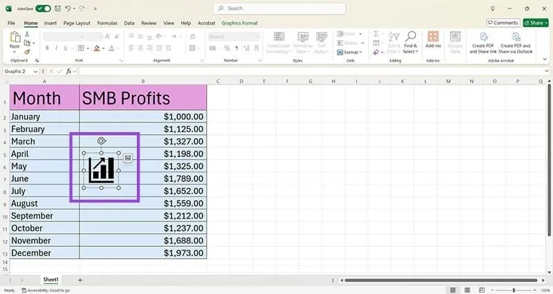
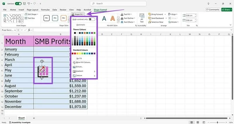
Step 5: To edit the icon color, go to the Graphics Format tab.
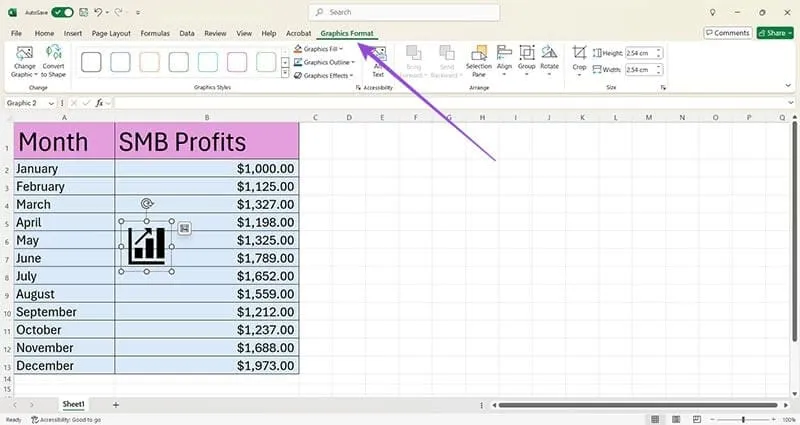
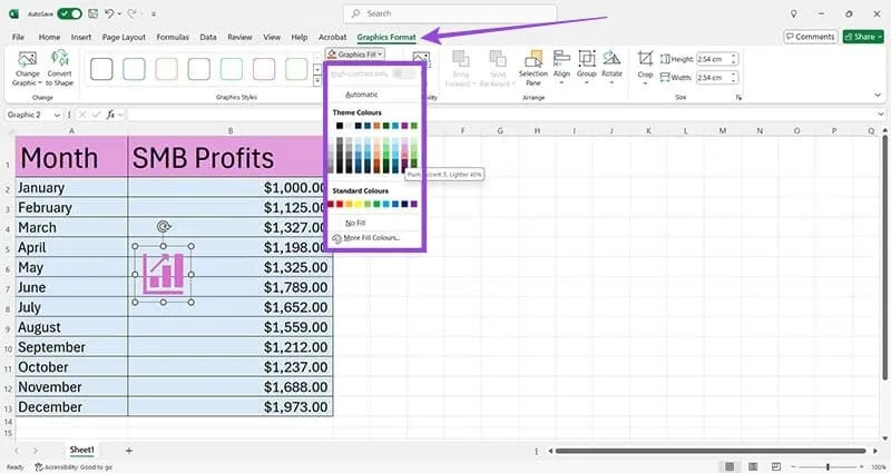
Step 6: Change the color via the dropdown menu next to Graphics Fill.
Step 7: To use multiple colors, convert the icon to a shape using the Convert to Shape option in the Graphics Format tab.
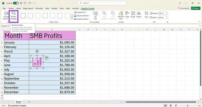
Step 8: Now you can customize colors for each part of the shape and resize it using the handles.
